homework_1 (Reproduce Figure 1b from Baggerly and Coombes (2009))

Figure description

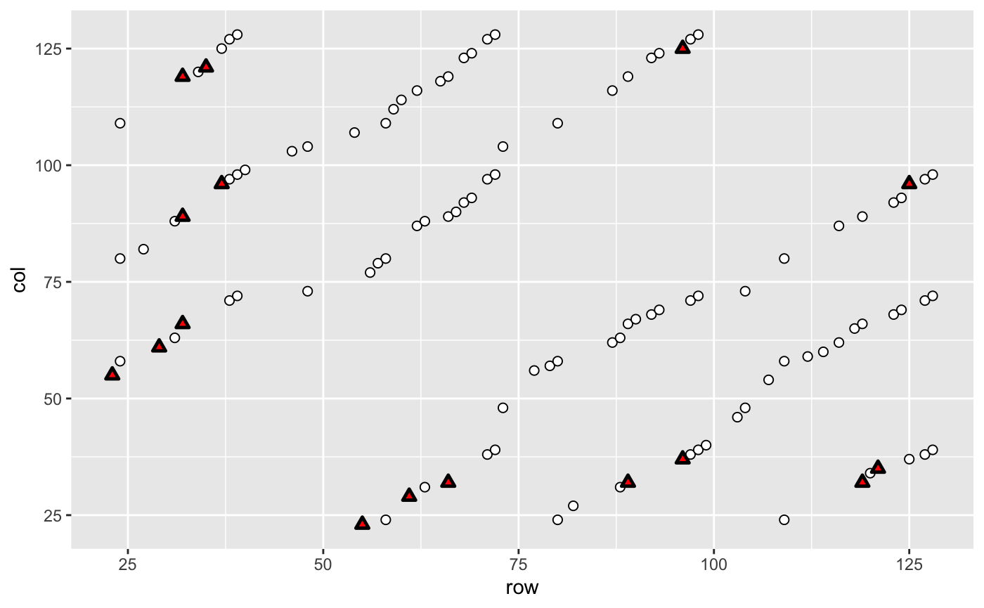
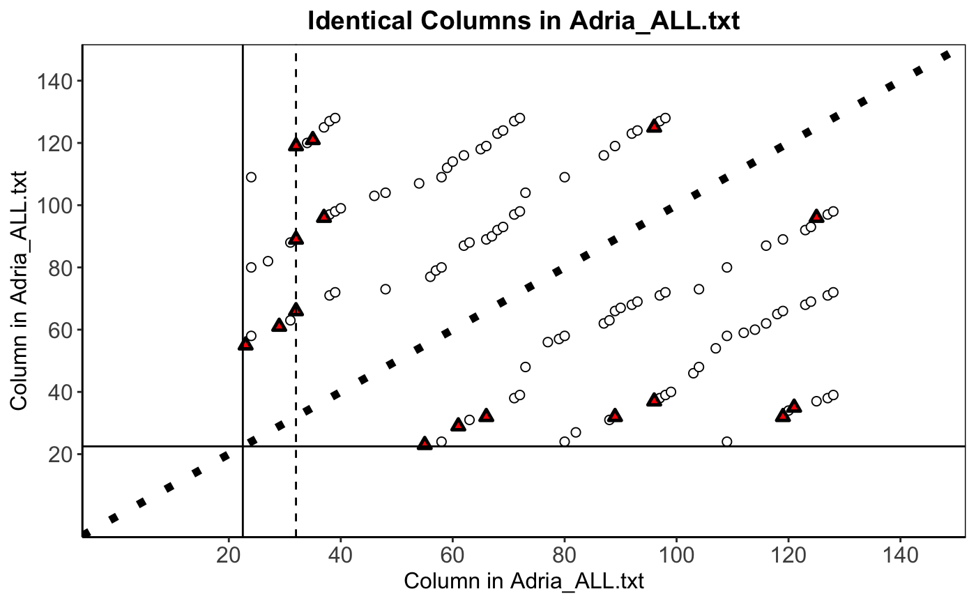
In order to get a more precise idea of the extent of the duplication, Baggerly and Coombes (2009) examined all pairwise sample correlations for Adria_ALL.txt. Figure 1(b) highlighted pairs with correlations above 0.9999 (duplicates). Circles indicated duplicates with consistent labels; triangles indicated duplicates where the same sample was labeled sensitive in one column and resistant in the other.

Reproduction

To reproduce this figure, we read the data “Adria_ALL.txt” first. This file contains 144 samples (22 training samples and 122 validation samples). There are two header rows. The first Row indicates whether the column is training (Adria) or testing (Validation). The second row indicates whether the column is Sens or Resistant (training) or Resp or NR (testing). In the training set, 0 denotes resistant and 1 denotes sensitive. There are 10 columns labeled as resistant, and 12 columns labeled as sensitive. The test (validation) data is all labeled 2, regardless of status. The test data contains 99 NR (resistant) samples and 23 Resp (sensitive) samples.

We read the first row as column names and rename the columns. Meanwhile, we save the second row as sample labels to a new data frame. And the labels in training and test are inconsistent, we rename “NR” as “Resistant”, “Sens” as “Sensitive” and “Resp” as “Sensitive”. Then we calculate the pairwise sample correlations, and save the pairs with correlations above 0.9999.

Next, we need to check the distant columns. We create a 144×144 matrix using the label data we created and find the consistent and inconsistent columns in high correlation pairs.

Now, we could reproduce the dotplot to identify identical columns in the full Adria_ALL.txt matrix. First, we add consistent (circles) and inconsistent (triangles) points to the plot.

Second, we add two reference lines to separate the training and test data, and marked a sample 32 with a dashed line. Because it is a good inconsistent example (sample 32 (main diagonal) is labeled “Resp,” but samples 66, 89, and 117 are labeled “NR” (triangles)). Last, we modify the themes, titles and axis. The following is the final version of this figure.

Appendix

par(mfrow=c(1,1))
library(dplyr)
library(ggplot2)

# Read data 
arida <- read.delim("Adria_ALL.txt",header = TRUE)
# Rename the column
adria_all <- read.table(file.path("Adria_ALL.txt"), sep = "\t", skip = 2, header = FALSE)
names<-c(paste("Training", c(1:22), sep = ""), paste("Test",c(1:122), sep = ""))
colnames(adria_all) <- names
adria_all[1:6, c(1:2, 22:25)]
#Create the samples labels
label_sample <- read.table(file.path("Adria_ALL.txt"), sep = "\t", skip = 1, nrows = 1, header = FALSE)

label_sample <- t(label_sample)%>%as.data.frame()%>%dplyr::mutate(V1=case_when(V1=="NR"~"Resistant",
                                                             V1=="Sens"~"Sensitive",
                                                             V1=="Resp"~"Sensitive",
                                                             TRUE~V1))
label_data <- data.frame(label= label_sample, row.names = names)

#calculate correlations, and save the correlations above 0.9999. 
adria_cor <- cor(adria_all)
adria_cor_high <- (adria_cor > 0.9999)

#check the distant columns
label_matrix <- matrix(rep(label_data[,"V1"], 144),144, 144)
label_same <- (label_matrix == t(label_matrix))
consistent <- which(adria_cor_high & label_same, arr.ind = TRUE)
consistent <- consistent[consistent[, 1] != consistent[, 2],] %>%as.data.frame()
inconsistent <- which(adria_cor_high & (!label_same),arr.ind = TRUE)%>%as.data.frame()

#reproduce the plot
p<-ggplot()+
  geom_point(consistent,mapping = aes(row, col), shape=21, fill="white",size=2)+
  geom_point(inconsistent,mapping = aes(row, col), shape=24, fill = "red",stroke = 1.3)
p<-p+scale_y_continuous(breaks=seq(20,140,20),limits=c(0.5,144.5))+
  scale_x_continuous(breaks=seq(20,140,20),limits=c(1,144.5))+
  geom_hline(yintercept = 22.5)+
  geom_vline(xintercept = 22.5)+
  geom_abline(intercept = 0, slope = 1,size = 2,linetype=21)+
  geom_vline(xintercept = 32, linetype = "dashed")+
  labs(title = "Identical Columns in Adria_ALL.txt",x= "Column in Adria_ALL.txt", y = "Column in Adria_ALL.txt")

p+theme_classic()+theme(plot.background = element_blank(),
        plot.title = element_text(size=14,face="bold",hjust=0.5),
        axis.title.x = element_text(size=12),
        axis.title.y = element_text(size=12),
        axis.text.x = element_text(size=12),
        axis.text.y = element_text(size=12),
        strip.background = element_rect(colour=NA,fill=NA),
        panel.border = element_rect(color="black",fill=NA))